Getting started with lbstproj • lbstproj

Introduction

This tutorial walks through a complete lbstproj workflow using a fake oncology project. We use the trial dataset - a simulated randomized clinical trial of 200 patients assigned to Drug A or Drug B - to demonstrate how to:

Scaffold a standardized project
Register outputs in the Table of Tables (TOT)
Write and run data preparation, figure, and table scripts
Generate a self-contained report

1. Create a project

create_project() builds the full directory structure and adds a DESCRIPTION file and a blank Table of Tables. We pass force = TRUE and open = FALSE to skip interactive prompts.

library(lbstproj)

create_project(
  path = tmp_proj_dir,
  title = "Fake oncology trial",
  client = "John Doe",
  department = "Oncology",
  author = "Jane Doe",
  email = "jane.doe@university.com",
  open = FALSE,
  force = TRUE
)

The project now has the following structure:

fs::dir_tree(tmp_proj_dir, recurse = TRUE)
#> /tmp/Rtmplb0h4L/fake-trial
#> ├── DESCRIPTION
#> ├── R
#> │   ├── data
#> │   ├── figures
#> │   ├── functions
#> │   └── tables
#> ├── data
#> │   ├── figures
#> │   ├── processed
#> │   ├── raw
#> │   ├── tables
#> │   └── tot
#> │       └── table_of_tables.xlsx
#> ├── docs
#> │   ├── costing.docx
#> │   └── meeting_notes.docx
#> ├── fake-trial.Rproj
#> ├── report
#> │   └── utils
#> └── results
#>     ├── figures
#>     ├── reports
#>     └── tables

Folder	Purpose
`data/raw/`	Raw input files (CSV, Excel, …)
`data/processed/`	Cleaned datasets saved as `.rds`
`data/tables/`	GT tables saved as `.rds`
`data/tot/`	The Table of Tables (Excel + cached `.rds`)
`R/data/`	Data preparation scripts
`R/figures/`	Figure scripts
`R/tables/`	Table scripts
`results/figures/`	Final PNG/PDF figures
`results/tables/`	Word tables (`.docx`)
`report/`	Quarto report

2. Import raw data

The trial dataset is bundled with lbstproj as a CSV. Copy it to data/raw/:

# In a real project you would place your raw data file in data/raw/ manually.
fs::file_copy("path/to/trial.csv", "data/raw/trial.csv")

trial_raw <- read.csv("data/raw/trial.csv")
head(trial_raw)
#>      trt age marker stage grade response death ttdeath
#> 1 Drug A  23  0.160    T1    II        0     0   24.00
#> 2 Drug B   9  1.107    T2     I        1     0   24.00
#> 3 Drug A  31  0.277    T1    II        0     0   24.00
#> 4 Drug A  NA  2.067    T3   III        1     1   17.64
#> 5 Drug A  51  2.767    T4   III        1     1   16.43
#> 6 Drug B  39  0.613    T4     I        0     1   15.64

The dataset has 200 patients with eight variables: treatment arm (trt), age, biomarker level (marker), tumour stage (stage), histological grade (grade), binary response, and survival endpoints (death, ttdeath).

3. The Table of Tables

The Table of Tables (TOT) is the central registry of every output your project will produce. It lives in data/tot/table_of_tables.xlsx and has four columns:

Column	Description
`id`	Short unique identifier (referenced inside scripts)
`type`	`"figure"` or `"table"`
`name`	File name used for saving (letters, numbers, hyphens only)
`caption`	Caption that appears in the report

For this project we plan two figures and two tables:

tot_data <- data.frame(
  id = c("fig-01", "fig-02", "tab-01", "tab-02"),
  type = c("figure", "figure", "table", "table"),
  name = c("fig-age-dist", "fig-km", "tab-baseline", "tab-response"),
  caption = c(
    "Age distribution by treatment arm.",
    "Kaplan-Meier curve of the survival over time per treatment arm.",
    "Baseline patient characteristics by treatment arm.",
    "Tumour response rates by treatment arm."
  ),
  stringsAsFactors = FALSE
)
tot_data
#>       id   type         name
#> 1 fig-01 figure fig-age-dist
#> 2 fig-02 figure       fig-km
#> 3 tab-01  table tab-baseline
#> 4 tab-02  table tab-response
#>                                                           caption
#> 1                              Age distribution by treatment arm.
#> 2 Kaplan-Meier curve of the survival over time per treatment arm.
#> 3              Baseline patient characteristics by treatment arm.
#> 4                         Tumour response rates by treatment arm.

After filling in the spreadsheet, call import_tot() to validate it and cache it as an .rds file:

import_tot()
#> ℹ Importing Table of Tables (TOT) to data/tot/tot.rds

You can always inspect the TOT with load_tot():

load_tot()
#> # A tibble: 4 × 4
#>   id     type   name         caption                                            
#>   <chr>  <chr>  <chr>        <chr>                                              
#> 1 fig-01 figure fig-age-dist Age distribution by treatment arm.                 
#> 2 fig-02 figure fig-km       Kaplan-Meier curve of the survival over time per t…
#> 3 tab-01 table  tab-baseline Baseline patient characteristics by treatment arm. 
#> 4 tab-02 table  tab-response Tumour response rates by treatment arm.

4. Create analysis scripts

create_from_tot() reads the TOT and generates stub R scripts for each entry. Always do a dry run first to preview what will be created:

create_from_tot(dry_run = TRUE)
#> 
#> ── Figures ──
#> 
#> ℹ Figures: 2 in TOT, 0 on disk, 0 matched.
#> ℹ Figures: would generate 2 missing programs.
#> → Figures: would create 2 programs in R/figures.
#> • R/figures/fig-age-dist.R
#> • R/figures/fig-km.R
#> 
#> ── Tables ──
#> 
#> ℹ Tables: 2 in TOT, 0 on disk, 0 matched.
#> ℹ Tables: would generate 2 missing programs.
#> → Tables: would create 2 programs in R/tables.
#> • R/tables/tab-baseline.R
#> • R/tables/tab-response.R

Once satisfied, run without dry_run to create the stubs:

create_from_tot(dry_run = FALSE)
#> 
#> ── Figures ──
#> 
#> ℹ Figures: 2 in TOT, 0 on disk, 0 matched.
#> ℹ Figures: generating 2 missing programs.
#> → Figures: created 2 programs in R/figures.
#> • R/figures/fig-age-dist.R
#> • R/figures/fig-km.R
#> 
#> ── Tables ──
#> 
#> ℹ Tables: 2 in TOT, 0 on disk, 0 matched.
#> ℹ Tables: generating 2 missing programs.
#> → Tables: created 2 programs in R/tables.
#> • R/tables/tab-baseline.R
#> • R/tables/tab-response.R

Each stub is pre-filled with a header, get_info() to retrieve TOT metadata, library calls, and placeholder comments:

#' Name         : fig-age-dist.R
#' Author       : Jane Doe
#' Date         : 03 Apr 2026
#' Purpose      :
#' Files created:
#'  - `results/figures/fig-age-dist.png/pdf`
#' Edits        :
#'  - 03 Apr 2026: Created file.

# File info ---------------------------------------------------------------

info <- get_info(name = "fig-age-dist")

# Packages ----------------------------------------------------------------

library(dplyr)
library(ggplot2)

# Load data ---------------------------------------------------------------

data <- NULL # Load processed data here

# Generate figure ---------------------------------------------------------

fig <- NULL # Replace NULL with your figure code, e.g. ggplot(data) + ...

# Save figure -------------------------------------------------------------

save_figure(fig, name = info$name)

You fill in the placeholder sections with your analysis. The next sections show the completed scripts for our oncology project.

5. Data preparation

All cleaning and reshaping happens in R/data/. The script below loads the raw CSV, coerces categorical variables to factors, and saves the result with save_data().

# R/data/trial-clean.R

library(dplyr)

# Load raw data ---------------------------------------------------------------
raw <- read.csv("data/raw/trial.csv")

# Clean -----------------------------------------------------------------------
trial <- raw |>
  mutate(
    trt = factor(trt),
    stage = factor(stage),
    grade = factor(grade, levels = c("I", "II", "III"))
  )

# Save ------------------------------------------------------------------------
save_data(trial, name = "trial-clean")

After running the script you can inspect the processed dataset:

trial <- readRDS("data/processed/trial-clean.rds")
dplyr::glimpse(trial)
#> Rows: 200
#> Columns: 8
#> $ trt      <fct> Drug A, Drug B, Drug A, Drug A, Drug A, Drug B, Drug A, Drug …
#> $ age      <int> 23, 9, 31, NA, 51, 39, 37, 32, 31, 34, 42, 63, 54, 21, 48, 71…
#> $ marker   <dbl> 0.160, 1.107, 0.277, 2.067, 2.767, 0.613, 0.354, 1.739, 0.144…
#> $ stage    <fct> T1, T2, T1, T3, T4, T4, T1, T1, T1, T3, T1, T3, T4, T4, T1, T…
#> $ grade    <fct> II, I, II, III, III, I, II, I, II, I, III, I, III, I, I, III,…
#> $ response <int> 0, 1, 0, 1, 1, 0, 0, 0, 0, 0, 0, 1, 0, 0, 0, 0, 1, 0, 0, 0, 0…
#> $ death    <int> 0, 0, 0, 1, 1, 1, 0, 1, 0, 1, 0, 0, 1, 1, 1, 1, 0, 1, 0, 0, 0…
#> $ ttdeath  <dbl> 24.00, 24.00, 24.00, 17.64, 16.43, 15.64, 24.00, 18.43, 24.00…

6. Figures

Figure 1 - Age distribution

# R/figures/fig-age-dist.R

library(dplyr)
library(ggplot2)

info <- get_info("fig-01")
trial <- readRDS("data/processed/trial-clean.rds")

fig <- ggplot(trial, aes(x = trt, y = age, fill = trt)) +
  geom_violin(alpha = 0.4, trim = FALSE) +
  geom_boxplot(width = 0.15, alpha = 0.8, outlier.shape = NA) +
  scale_fill_brewer(palette = "Set2") +
  labs(x = "Treatment arm", y = "Age (years)") +
  theme_minimal(base_size = 12) +
  theme(legend.position = "none")

save_figure(fig, name = "fig-age-dist", width = 5, height = 4)

#> Warning: Removed 11 rows containing non-finite outside the scale range
#> (`stat_ydensity()`).
#> Warning: Removed 11 rows containing non-finite outside the scale range
#> (`stat_boxplot()`).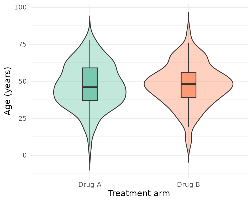

Age distribution by treatment arm.

Figure 2 - Kaplan-Meier curve

# R/figures/fig-km.R

library(dplyr)
library(ggplot2)
library(ggsurvfit)

info <- get_info("fig-02")
trial <- readRDS("data/processed/trial-clean.rds")

mod <- survfit2(
  data = data,
  formula = Surv(ttdeath, death) ~ response
)

fig <- ggsurvfit(mod) +
  add_confidence_interval() +
  labs(
    x = "Months since treatment",
    y = "Survival probability",
    color = "Tumor Response",
    fill = "Tumor Response"
  ) +
  theme_minimal(base_size = 12)

save_figure(fig, name = "fig-km", width = 5, height = 4)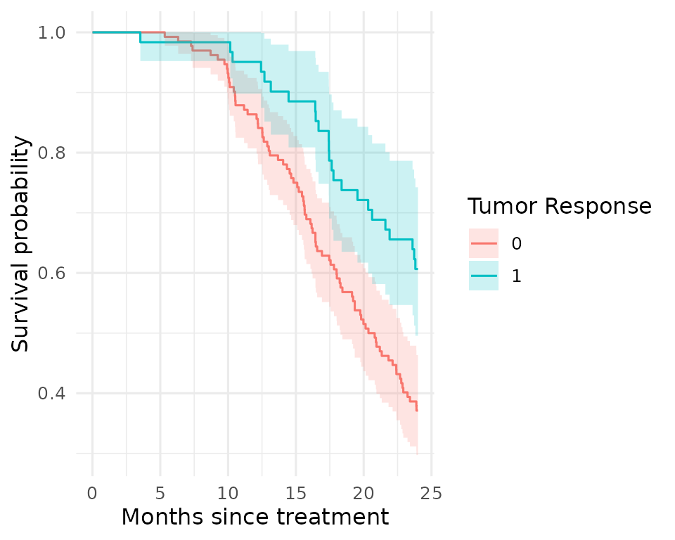

Tumour response rate by treatment arm.

7. Tables

Tables are saved as gt objects and optionally exported to Word. The workflow below uses gtsummary to produce publication-ready summaries, then converts to gt with as_gt() before saving.

Table 1 - Baseline characteristics

# R/tables/tab-baseline.R

library(dplyr)
library(gtsummary)

info <- get_info("tab-01")
trial <- readRDS("data/processed/trial-clean.rds")

tab <- trial |>
  select(trt, age, stage, grade) |>
  tbl_summary(
    by = trt,
    label = list(
      age ~ "Age (years)",
      stage ~ "Tumour stage",
      grade ~ "Grade"
    )
  ) |>
  add_overall() |>
  add_p() |>
  modify_header(label ~ "**Characteristic**") |>
  bold_labels() |>
  as_gt() |>
  gt::tab_header(title = info$caption)

save_table(tab, name = "tab-baseline", export = FALSE)

readRDS("data/tables/tab-baseline.rds")

Characteristic	Overall N = 200¹	Drug A N = 98¹	Drug B N = 102¹	p-value²
Baseline patient characteristics by treatment arm.
Age (years)	47 (38, 57)	46 (37, 60)	48 (39, 56)	0.7
Unknown	11	7	4
Tumour stage				0.9
T1	53 (27%)	28 (29%)	25 (25%)
T2	54 (27%)	25 (26%)	29 (28%)
T3	43 (22%)	22 (22%)	21 (21%)
T4	50 (25%)	23 (23%)	27 (26%)
Grade				0.9
I	68 (34%)	35 (36%)	33 (32%)
II	68 (34%)	32 (33%)	36 (35%)
III	64 (32%)	31 (32%)	33 (32%)
¹ Median (Q1, Q3); n (%)
² Wilcoxon rank sum test; Pearson’s Chi-squared test

Table 2 - Response rates

# R/tables/tab-response.R

library(dplyr)
library(gtsummary)

info <- get_info("tab-02")
trial <- readRDS("data/processed/trial-clean.rds")

tab <- trial |>
  select(trt, response) |>
  mutate(
    response = factor(response, levels = c(1, 0), labels = c("Yes", "No"))
  ) |>
  tbl_summary(
    by = trt,
    label = list(response ~ "Tumour response")
  ) |>
  add_p() |>
  modify_header(label ~ "**Variable**") |>
  bold_labels() |>
  as_gt() |>
  gt::tab_header(title = info$caption)

save_table(tab, name = "tab-response", export = FALSE)

readRDS("data/tables/tab-response.rds")

Variable	Drug A N = 98¹	Drug B N = 102¹	p-value²
Tumour response rates by treatment arm.
Tumour response	28 (29%)	33 (34%)	0.5
Unknown	3	4
¹ n (%)
² Pearson’s Chi-squared test

8. Running all outputs

Once all scripts are written, run_all_figures() and run_all_tables() source every script in R/figures/ and R/tables/ in alphabetical order. They also cross-check the file list against the TOT and warn you about any discrepancies.

run_all_figures()

run_all_tables()

9. Generating the report

Create the report scaffold

create_report() reads the TOT and generates a Quarto file at report/report.qmd with a code chunk for every figure and table, in the order they appear in the TOT.

create_report(output_type = "html")

#> ✔ Writing report to report/report_2026_04_03.qmd.
#> ℹ Use `run_report()` to render the report.

The generated file looks like this (excerpt):

---
title: "Fake oncology trial"
subtitle: "John Doe (Oncology)"
author: "Jane Doe"
date: last-modified
format:
  html:
    embed-resources: true
    toc: true
    toc-location: left-body
    number-sections: true
execute:
  echo: false
  warning: false
  message: false
---

```{r pkg}
library(here) # To generate relative file paths
library(gt) # Needed to display gt tables in Word

# Create list of captions
tot <- readRDS(here("data/tot/tot.rds"))
caption_list <- setNames(as.list(tot$caption), tot$name)

# Define function to add caption to tables
add_caption <- function(x, cap) {
  x |>
    gt::tab_header(NULL) |>
    gt::tab_caption(cap)
}
```

```{r fig-fig-age-dist }
#| fig-cap: !expr 'caption_list[["fig-age-dist"]]'

knitr::include_graphics(here("results/figures/fig-age-dist.png"))
```

Render the report

Call run_report() to render the Quarto file to HTML (or DOCX):

run_report()

After reviewing the HTML report, archive it to results/reports/ with a date-stamped filename using archive_report():

archive_report()

Summary

Here is the full lbstproj workflow at a glance:

library(lbstproj)

# 1 - Scaffold the project
create_project(path = ".", title = "My project", author = "Jane Doe")

# 2 - Fill in data/tot/table_of_tables.xlsx, then import it
import_tot()

# 3 - Generate script stubs for every TOT entry
create_from_tot(dry_run = FALSE)

# 4 - Fill in the scripts, then run them all
run_all_files("data")
run_all_figures()
run_all_tables()

# 5 - Build and render the report
create_report(output_type = "html")
run_report()
archive_report()